Triton Kernel Profiling with Proton and ROCm on AMD GPUs

This is the second article in our series on Triton kernel profiling. In our first post, Triton kernel profiling with NVIDIA Nsight tools, we introduced how to profile and optimize custom Triton GPU kernels on NVIDIA hardware. In this post, we focus specifically on optimizing performance for AI and machine learning workloads on AMD GPUs. Understanding why a kernel is performing a certain way is the first step toward writing better, faster code. This article introduces two powerful profiling tools—Triton Proton and the ROCm Compute Profiler—that can help developers unlock the full potential of their GPU kernels on AMD GPUs.

The Triton Proton profiler and the ROCm Compute Profiler play distinct but complementary roles in the overall analysis. Triton Proton is a lightweight, vendor-agnostic profiler designed specifically for Triton kernels. It provides essential information about program context, metadata, and general hardware performance metrics, serving as a starting point to identify general performance issues or “hot spots.” The ROCm Compute Profiler, on the other hand, is a comprehensive, vendor-specific (for AMD GPUs) kernel-level tool. It offers greater specificity and useful hardware information, including detailed hardware counter statistics, making it ideal for providing the necessary data to resolve the specific hot spots identified by Proton. By using both tools, developers gain a complete picture: Proton gives the broad, initial diagnosis, and ROCm Compute Profiler provides the deep, vendor-specific detail needed for ultimate optimization.

Key takeaways

By the end of this guide, you will know:

• How to get started using the Triton Proton profiler to perform a vendor-agnostic analysis of a Triton GPU kernel’s performance.
• How to get started using the ROCm Compute Profiler to perform a vendor-specific analysis of a Triton GPU kernel, uncovering detailed hardware performance data.

Red Hat’s Emerging Technologies blog includes posts that discuss technologies that are under active development in upstream open source communities and at Red Hat. We believe in sharing early and often the things we’re working on, but we want to note that unless otherwise stated the technologies and how-tos shared here aren’t part of supported products, nor promised to be in the future.

Resources

To follow along with this guide, you will need the following:

• Source:
  • Triton profiling blog repository
    • Jupyter notebook
    • Jupyter notebook HTML
• Information:
  • Proton manual
  • ROCm compute profiler documentation
• Hardware:
  • An AMD GPU, such as an MI300X or newer enterprise grade AMD GPU.
    • This hardware is required only to run the steps yourself. The notebook and exported files provide the output from all steps used to gather the data used in this blog.

Setup

Here are the basic steps to get your environment ready to run the notebook:

1. Setup AMD GPU host: Ensure you have the necessary prerequisites installed:

• ROCm 7.0
• Docker or Podman

2. Clone the blog-triton-profiling repository:

git clone https://github.com/redhat-et/blog-triton-profiling

3. Run the ROCm Jupyter Notebook container: This automatically launches a Jupyter Notebook lab server, which you can use to open and run the MatrixMultiplicationBias notebook.

cd blog-triton-profiling
make rocm-jupyter

4. Run the ROCm console container: Use this to access the command line within the profiling environment, which is necessary for running the profiler tools directly.

cd blog-triton-profiling
make rocm-console

Using Proton

Proton provides a simple and flexible way to obtain basic kernel performance metrics. As a lightweight profiler for Triton kernels, it offers a straightforward means of acquiring essential information such as program context, metadata, and hardware performance metrics. Developers can use Proton in two ways: either as a simple command-line tool to analyze a Triton program or by integrating its API directly into the Triton application code for more granular control over the metrics gathered. Regardless of the method, Proton also includes a viewer tool to display the resulting metrics that can also be used as a command-line tool or used as part of the Triton application code.

Command-line tools

To analyze a Triton program using the command line, run the proton tool with the command: proton --context python --data tree  --name <results filename> <program to profile>. To analyze the resulting hatchet file, the proton-viewer tool is used. You can list the available metrics with proton-viewer --list <filename>.hatchet, or you can print specified profile metric data (e.g., flops16, time/s) with proton-viewer --metrics <metrics separated by ,> --format full <filename>.hatchet.

Adding Proton to your Triton program

For more control, Proton can be integrated directly into the Triton application code. To collect a Proton report file (hatchet file), you need to write a kernel launch metadata function to collect the desired kernel data from the kernel’s inputs. Then, import the Python Proton module and use the profiler API as shown in the example code below.

import triton.profiler as proton
def kernel_launch_metadata(grid, kernel, args):
# ...
@triton.jit(launch_metadata=kernel_launch_metadata)
def triton_kernel( # ... )
# __main__
proton.start( # ... )
# ... run your kernel
proton.finalize()

After collecting the report, results can be analyzed using the viewer API: import triton.profiler.viewer as proton_viewer... (Code examples for this integration are available in the accompanying Jupyter notebook).

Using ROCm Compute

The ROCm Compute profiler offers deep, vendor-specific hardware information for analyzing your kernels.

You begin the process by running the rocprof-compute profile -n <profile name> -- <program and arguments> command to analyze your Triton kernel. Once the profile data is collected, you can proceed to analyze the results using the rocprof-compute analyze -p <path to profile data> command, which supports several output formats.

For a visual analysis, you can use the Graphical User Interface (GUI) with the command rocprof-compute analyze -p <path to profile data> --gui [port], where the port argument is optional. Alternatively, you can output a report directly to the console by running rocprof-compute analyze -p <path to profile data>. This command will output kernel information, system information, and general utilization metrics, which is useful for quickly dumping results into the output cell of a Jupyter notebook. For users working on remote machines via a terminal, the Terminal User Interface (TUI) is ideal, accessed with rocprof-compute analyze -p <path to profile data> --tui.

Finally, a crucial feature for post-analysis and exploration is the ability to list available metrics, which is done using the command rocprof-compute analyze -p <path to profile data> --list-metrics <GPU name, i.e. gfx90a>. This allows you to load and explore performance data even without an MI300 series GPU available for a live run.

Analysis

Note: All profiling metrics discussed in the following sections were gathered on an AMD MI300X GPU.

The Triton Proton profiler and the ROCm Compute Profiler play distinct but complementary roles in the overall analysis:

• Triton Proton Profiler: A vendor-agnostic tool providing basic kernel performance metrics and context. Used for initial identification of general performance issues or “hot spots.”
• ROCm Compute Profiler: An AMD-specific tool offering detailed, comprehensive kernel-level profiling and hardware counter statistics. It uses detailed hardware data to resolve specific hot spots identified by Proton.

By using both tools, developers gain a comprehensive picture: Proton gives the broad, initial diagnosis, and ROCm Compute Profiler provides the deep, vendor-specific detail needed for ultimate optimization.

Profiler metrics

Proton analysis

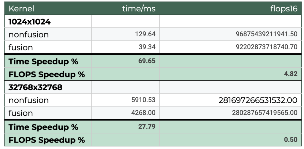
^{Table 1. Triton Proton Profiler metrics and speedup % between the profiled kernels}

The Triton Proton profiling metrics provide a vendor-agnostic view into the performance characteristics of the non-fusion and fusion kernels. This analysis focuses on the Floating-Point Operations Per Second (FLOPS) and total runtime to identify the primary performance bottleneck and quantify the benefits of kernel fusion for both small and large input sizes.

The analysis confirms that the kernels are load-bound, meaning their performance bottleneck is rooted in data movement and kernel launch overhead rather than raw computational power. This is evident from the highly consistent FLOPS across both kernel types and input sizes, with only a 4.82% difference for the small input and a negligible 0.50% difference for the large input.

By examining the runtime, we can pinpoint the primary bottleneck for different input sizes. For the small input (1024×1024), launch overhead is the primary bottleneck. Kernel fusion provides a dramatic 69.65% time speedup by eliminating the overhead of loading multiple kernels, requiring only a single fused kernel launch. Conversely, for the large input (32768×32768), data load time is the dominant factor. Fusion still yields a significant 27.79% time speedup by reducing kernel launch overhead, but the overall percentage improvement is lower than the small input case because the increased time to load the large input data becomes a more dominant factor in the total runtime.

In conclusion, the consistent FLOPS across all tests solidifies the finding that performance is bottlenecked by data loading and kernel launch overhead, not raw computational power. The fused kernel consistently reduces runtime by lowering the overhead of loading multiple kernels. This effect is most pronounced with small inputs where launch overhead is the dominant factor, while the analysis of the larger input size provides a more representative picture of the improvement where the greater impact of data load time on the total runtime naturally results in a lower overall percentage speedup.

ROCm Systems Compute Analysis

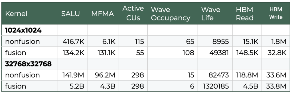
^{Table 2. Some selected metrics taken from the ROCm Compute Profiler results}

On the other hand, ROCm Compute Profiler gives us a deeper look into the workings of the hardware. We can use it to examine hardware counters, memory bandwidth utilization, and much more. In this section, we will discuss how to interpret HBM and different ALU utilization rates and how to interpret them in relation to performance. 

The performance profile of small input matrices (1024×1024) in non-fused environments is primarily throttled by execution overhead and inefficient hardware utilization. In unfused workflows, the system relies heavily on the scalar ALU (SALU), which leads to suboptimal Matrix Fused Multiply-Add (MFMA) utilization and suboptimal memory usage patterns. High High-Bandwidth Memory (HBM) utilization is limited by this behavior; repeated read/write cycles of intermediate data, combined with the high dispatch overhead of serially launched kernels for small jobs, creates significant latency. By contrast, kernel fusion optimizes these workloads by prioritizing matrix cores (MFMA) and reducing scalar (SALU) instruction counts.

Fusion significantly mitigates the “memory wall” even for small inputs by utilizing the GEMM output as a tiled intermediary matrix. This allows the bias and matrix multiplication stages to consume data directly from the registers or cache rather than performing serial reloads from global memory. Additionally, the reduction in kernel launch overhead and the minimization of HBM write-backs allow the compute units to remain active longer. For small-scale inputs, this reduction in launch overhead is the dominant factor in runtime improvement, leading to a much higher effective throughput than the non-fused equivalent.

For large-scale inputs (32768×32768), the performance bottlenecks shift from launch overhead toward memory bandwidth saturation. In non-fused scenarios, the compiler still favors scalar operations slowing the system down overall, and the kernel still suffers from bandwidth thrashing on reading and writing the intermediate data. In this case, poor HBM utilization throttles the kernel more than the kernel launch overhead. The HBM remains underutilized because a large portion of that bandwidth is dedicated to redundant data movement. It also does not use vectorized instructions, which are favored by the MFMA. Overall, this leads to a read speed being over 37 times faster on the fused vs nonfused kernel.

Applying fusion to large inputs results in substantial speedups by optimizing data load statistics as well as compute utilization. While the raw FLOPs remain relatively consistent (see the table in Proton analysis), indicating that the compute logic is already saturated, the fused kernels significantly improve the read/write efficiency. By reusing memory space within a single, longer kernel, the system avoids the cycles of thrashing that characterize unfused executions. Ultimately, the transition from an I/O-bound state to a more compute-bound state allows the hardware to maintain higher utilization across the entire duration of the workload, showing that fusion is critical for both overhead reduction in small tasks and memory bandwidth optimization in large-scale processing.

Conclusion

By using both the Triton Proton Profiler and the ROCm Compute Profiler, you gain a comprehensive picture of your kernel performance. Proton gives a vendor-agnostic view of basic kernel performance metrics to initially identify general performance issues or “hot spots,” while vendor-specific tools like the ROCm Compute Profiler provide much greater specificity and useful hardware information, which can be used to resolve the hot spots identified by Proton.

Through this combined approach, we analyzed non-fusion vs. fusion kernel performance and found that a fused kernel provides significant performance improvements. This is because all the work is done within a single kernel, resulting in improved launch overhead and better pipeline saturation. Conversely, a non-fusion kernel struggles to saturate the pipeline as the work is broken into smaller chunks, making performance often dominated by launch overhead.

Call to action

Dive deeper into Triton kernel optimization and try the examples yourself! Clone the Triton Profiling Blog Repository today to access the full Jupyter Notebook.

Additional resources

• Democratizing AI accelerators and GPU kernel programming using Triton
• Getting started with PyTorch and Triton on AMD GPUs using the Red Hat Universal Base Image
• A container-first approach to Triton development
• Understanding Triton cache: optimizing GPU kernel compilation
• From hand-tuned to generated: areproducible Triton GPU kernel benchmark across different vendors
• Triton kernel profiling with NVIDIA Nsight tools