
Are your custom Triton GPU kernels running as efficiently as they could be? Unlocking peak performance requires the right tools. This blog post is all about diving into profiling a Triton GPU kernel, with a specific focus on compute performance, using the powerful NVIDIA Nsight Tools. So, what exactly are these tools? NVIDIA Nsight Systems is a powerful system-wide performance analysis tool that helps you visualize and optimize the overall application workflow, identifying bottlenecks and areas for improvement. NVIDIA Nsight Compute, on the other hand, is a GPU kernel profiler that provides detailed performance metrics and insights at the kernel level, helping you understand and optimize individual GPU computations. We will be focusing on NVIDIA Nsight Compute for this post.
What is a GPU kernel? In simple terms, a GPU kernel is a function that runs on a GPU, typically executing in parallel across many threads. For more in-depth information, you might find other resources that specifically cover GPU kernel fundamentals. And what about Triton? Triton is a high-level language and compiler designed specifically for writing highly efficient custom GPU kernels, particularly for neural networks.
Red Hat’s Emerging Technologies blog includes posts that discuss technologies that are under active development in upstream open source communities and at Red Hat. We believe in sharing early and often the things we’re working on, but we want to note that unless otherwise stated the technologies and how-tos shared here aren’t part of supported products, nor promised to be in the future.
Key Takeaways
In this article, you will learn:
- How to get started using NVIDIA Nsight Compute to analyze the performance of a Triton GPU kernel.
- How to identify performance bottlenecks, such as memory-bound versus compute-bound operations.
- How Triton’s autotuning feature can be used to test configurations and significantly improve kernel performance.
Resources
To follow along or explore further, here are some helpful resources:
- Triton: Learn more about Triton at https://triton-lang.org/main/index.html.
- Tools:
- Our accompanying code and workspace can be found at https://github.com/redhat-et/blog-triton-profiling. Specifically, check out `workspace/MatMul.jpynb` for the Triton Kernel example.
- An overview of the NVIDIA Nsight tools: https://developer.nvidia.com/tools-overview.
- For Nsight Systems, learn more at https://developer.nvidia.com/nsight-systems.
- For Nsight Compute, learn more at https://developer.nvidia.com/nsight-compute.
- Operating System: We are using Fedora 42 (https://fedoraproject.org) to run the containers found in the provided code.
- Container Runtime: We are using Podman (https://podman.io).
- Hardware: An NVIDIA GPU, such as an RTX 4070 or RTX 5000 Ada. This is required to run the kernel and profile it.
Setup
Follow these guides to ensure the host is set up correctly.
- NVIDIA GPU Driver Installation Guide
- https://docs.nvidia.com/datacenter/tesla/driver-installation-guide/index.html
- Alternative method: Using the driver packages from RPMFusion (https://rpmfusion.org/Howto/NVIDIA?highlight=%28%5CbCategoryHowto%5Cb%29)
- NVIDIA Container Toolkit Installation Guide
- Instructions to fix GPU Performance Counters user permissions for Nsight Compute
Getting started with our demo is straightforward:
1. Get the demo source:
git clone https://github.com/redhat-et/blog-triton-profiling
2. Let’s run Jupyter Notebook to look at the Triton kernel:
Use make cuda-jupyter to start a local Jupyter Notebook Lab.
When the command completes, you will get the URL for the server, which can be opened in your local browser

After opening the link in your browser, you should be greeted with this screen:
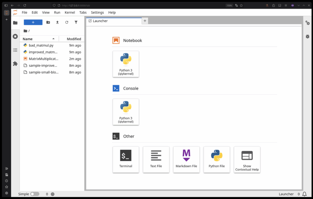
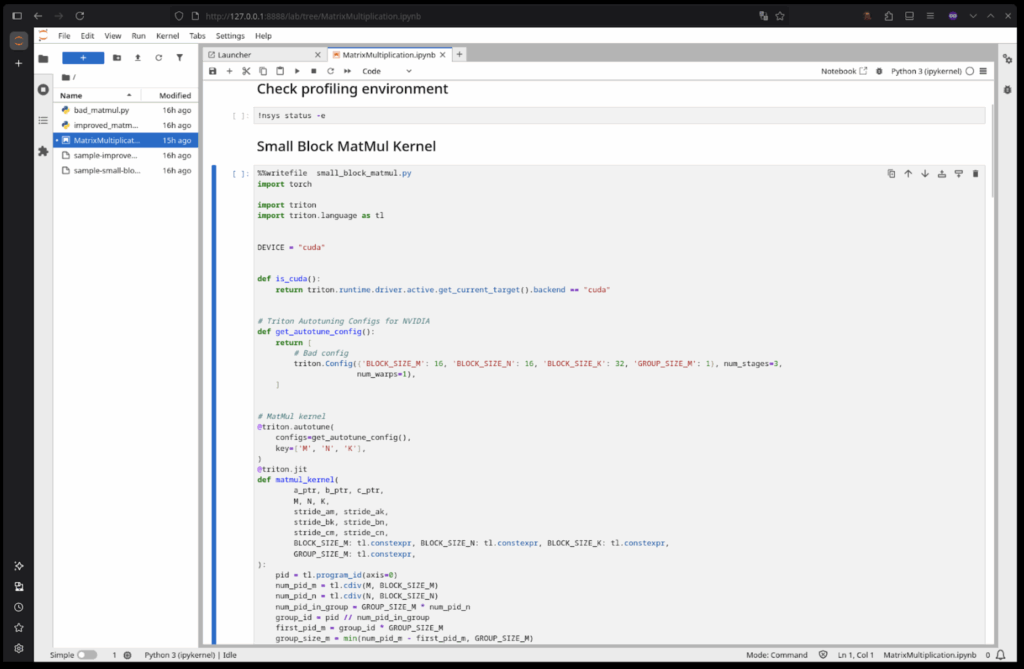
Double-click the MatrixMultiplication.ipynb notebook from the file browser on the left and it will open the Triton kernel.

Use Ctrl + C in the terminal window you ran the make cuda-jupyter command in to shutdown the server.
3. Let’s run Nsight Compute to view the reports from the demo:
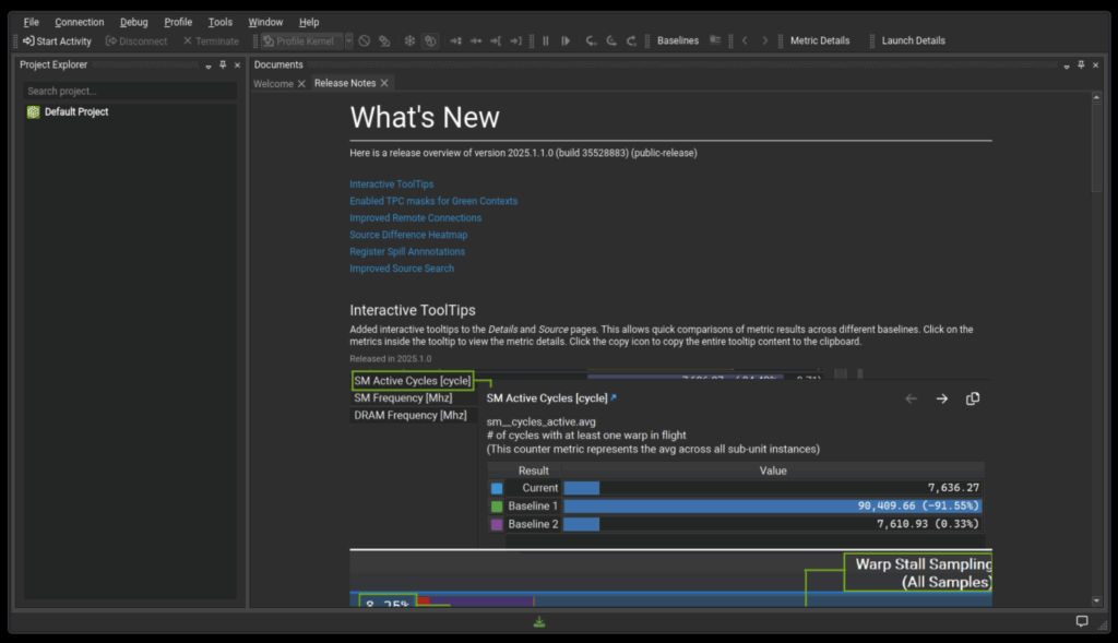
Use make cuda-compute to launch the Nsight Compute UI. It will look like this after you say Yes or No to the analytics collection dialog.
Open the report by selecting “File -> Open File”, which will open the file browser at /workspace.
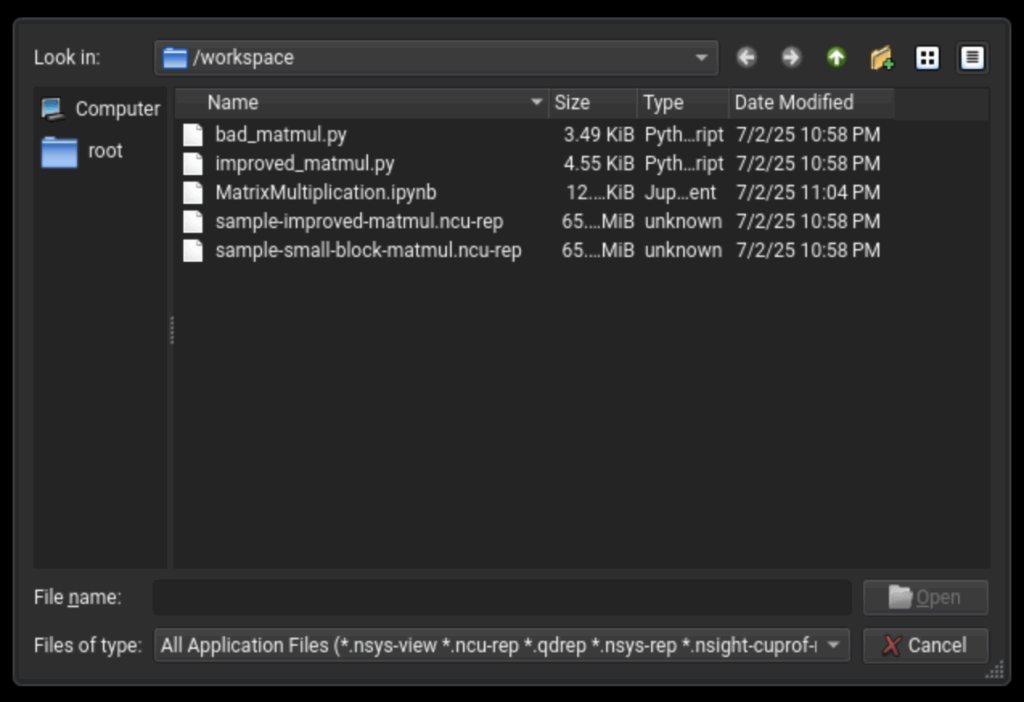
You can open both Compute, “<filename>.ncu-rep”, files and Systems, “<filename>.nsys-rep” files in the Nsight Compute UI app.
Additional commands:
- Use
make cuda-systemsto launch the Nsight Systems UI. - Use
make cuda-consoleto launch a shell inside a container. - Use
make nsight-systemsto launch the Nsight Systems UI without a GPU - Use
make nsight-computeto launch the Nsight Compute UI without a GPU
Note: Each command runs a new container that will be removed when it exits.
Setup Video Demo
Profiling a Triton GPU Kernel
Let’s walk through the core of our profiling journey.
First, let’s get an overview of the Triton kernel we’ll be profiling. You can find the specific example in MatrixMultiplication.ipynb. It is based on the Triton tutorial Matrix Multiplication (MatMul) kernel.
Block processing algorithm
accumulator = tl.zeros((BLOCK_SIZE_M, BLOCK_SIZE_N), dtype=tl.float32)
for k in range(0, tl.cdiv(K, BLOCK_SIZE_K)):
    a = tl.load(a_ptrs, mask=offs_k[None, :] < K - k * BLOCK_SIZE_K, other=0.0)
    b = tl.load(b_ptrs, mask=offs_k[:, None] < K - k * BLOCK_SIZE_K, other=0.0)
    accumulator = tl.dot(a, b, accumulator)
    a_ptrs += BLOCK_SIZE_K * stride_ak
    b_ptrs += BLOCK_SIZE_K * stride_bk
The above section of the kernel handles most of the loading and actual mathematical operations of the kernel. Importantly we reserve our workspace in the accumulator that is defined as the size of BLOCK_SIZE_M x BLOCK_SIZE_N. The workspace size for each section of the matrix multiply operation is a tunable parameter that we will get into more later. Then, within the loop, we load a slice of input matrices A and B, in variables a and b, with each slice being BLOCK_SIZE_K in size. The for loop progresses through each matrix in this manner.
Now you may notice the sizes of BLOCK_SIZE_K/M/N are left undefined in the kernel. The parameters for block size are defined outside the function in a kernel configuration block. We will run with two blocks for this example, one with minimum size blocks and the other with the more optimal block sizes from a process called tuning. First the small configuration:
Small configuration
triton.Config({'BLOCK_SIZE_M': 16, 'BLOCK_SIZE_N': 16, 'BLOCK_SIZE_K': 32, 'GROUP_SIZE_M': 1}, num_stages=3, num_warps=1),
In this configuration we will have a workspace of size 16×16, loading slices of size 32 with a mask. Each of these sizes are in elements multiplied by size of the data type. So in this case if we look at the load of a, we get a block only 16 values wide. Due to this we don’t load the full elements from BLOCK_SIZE_K and we do very small, repeated loads. You may notice this is not efficient and using Nsight Compute we can quantify how inefficient it is. To capture this data, run the through the Jupyter notebook by following the steps below:
1. Select the Small Block MatMul Kernel cell and run it
2. Next select the Profile the Small Block MatMul Kernel cell

3. Open the resulting small-block-matmul.ncu-rep using the Nsight Compute UI
The same steps as above can be followed for profiling the Improved MatMul Kernel cell and accompanying Profile the Improved MatMul Kernel, which will generate a similar report file named improved-matmul.ncu-rep.
There are sample report files contained in the source repository, the following sections use those reports.
NOTE: The sample-improved-matmul.ncu-rep report file contains only the results from a single auto-tune configuration, the improved-matmul.ncu-rep report file that is generated by the notebook will show the matmul_kernel being run multiple times as it will have multiple runs for each auto-tune config due to the auto-tuner running through them to find the best configuration. For future runs, Triton would select the best fit kernel and run just that one.
When viewing the sample-small-block-matmul.ncu-rep report file from a run of just the small block tuning config you get the following:
Small Block Size Kernel Report

The key metrics to note here are the compute throughput and the memory throughput. We can see here that this kernel looks like it is memory bound since the compute throughput is so much lower than the memory throughput. Looking at it through that lens, we see that the L1 and L2 memory throughput are not fully utilized and that implies we are not fully taking advantage of our low level memory. In most cases this further implies that we are struggling with unoptimized load behavior. Here, the cause of the inefficiency is clear: we are loading small blocks with high frequency. While we intuitively know matrix multiplication tends to be compute-bound, the root cause of a bottleneck isn’t always this obvious.
Triton kernels can have kernel configuration properties flagged in a way that tells the Triton compiler to try all listed variations to find the fastest kernel. In this way we can let Triton itself test variations to find local performance maximums for various block and input sizes in a way that gets us close to optimal with very little time and only requiring human effort in setting bounds to the testing space. To see the list of configurations for these kernels, please reference the Triton Autotuning Configs for NVIDIA comments found in both the Small Block MatMul Kernel and Improved MatMul Kernel cells found in MatrixMultiplication.ipynb.
Running all the listed configurations given there and taking the best configuration found by Triton we get the following improved configuration:
Improved configuration
triton.Config({'BLOCK_SIZE_M': 128, 'BLOCK_SIZE_N': 256, 'BLOCK_SIZE_K': 64, 'GROUP_SIZE_M': 8}, num_stages=3, num_warps=8),
If we profile this configuration as we did above we get the following report (sample-improved-matmul.ncu-rep):
Improved Kernel Report
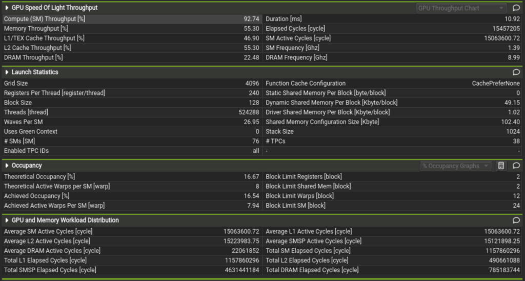
Note the duration went from 418.63 milliseconds to 10.92 milliseconds. We now also load the blocks for a and b in 64 element chunks of a 128×256 element block. Less wasted loading and better utilization of low level memory tells us that this is better but how do we know if it’s approaching optimal in this limited use case? Well, we can see now that Compute Throughput is at 92.74% and Memory Throughput is at 55.30%. This indicates that we are now compute-bound. For a low complexity kernel with little to no branching logic and linear memory loading of large blocks, this is expected behavior and we can assume this kernel will most likely scale with compute capacity. But thanks to Triton running autotuning on all platforms, this level of automatic optimization can be achieved on all other supported and future platforms as Triton itself is updated. Additionally since the Triton compiler bundles memory load optimization into the compile step, the user is left more able to focus on kernel logic. In turn, allowing for rapid prototyping and writing kernels that get close to using lower level languages.
Understanding the above, one can see how you could use Nsight Compute to optimize the auto-tune configurations for a Triton kernel. One caveat is that adding too many auto-tune configurations can increase the program runtime drastically as the auto-tuner will be running each one multiple times before selecting the best. As a result, it is better to keep the number of configurations limited per-run. To test a new configuration, profile a run of the kernel using only that configuration and compare it against previous profiles.
Conclusion
In conclusion, we’ve explored the power of NVIDIA Nsight Tools in dissecting and optimizing Triton GPU kernels. We’ve seen how Nsight Compute offers invaluable, detailed metrics at the kernel level. By leveraging these tools, we can identify performance bottlenecks, understand the impact of various kernel configurations, and ultimately achieve significant performance improvements. As AI and machine learning workloads become more demanding, the ability to fine-tune GPU kernels with this level of precision becomes a critical skill for any developer looking to maximize hardware efficiency.
Kernel Analysis Video Demo
To solidify your understanding, we have a short video demo:
Thank you for joining us on this journey into Triton kernel profiling!
Additional Resources
- Democratizing AI Accelerators and GPU Kernel Programming using Triton
- Getting started with PyTorch and Triton on AMD GPUs using the Red Hat Universal Base Image
- A container-first approach to Triton development
- Understanding Triton Cache: Optimizing GPU Kernel Compilation