
Quantum computing is an emerging paradigm in computer science which aims to bridge gaps in problems that classical computers, meaning those that follow the traditional deterministic model of computing, have difficulty solving. Building off of our previous post, “Quantum on OpenShift – part one, an introduction to quantum computing”, we will use this blog post to demonstrate how we can make quantum systems work for us through the use of an OpenShift 4 cluster. We will use Qiskit to develop our quantum circuits and execute them on top of IBM Quantum, a premier quantum computing laboratory. If you are running a Kubernetes cluster and would like to follow along, you can find a guide on installing QiskitPlayground here.
Note: Red Hat’s Emerging Technologies blog includes posts that discuss technologies that are under active development in upstream open source communities and at Red Hat. We believe in sharing early and often the things we’re working on, but we want to note that unless otherwise stated the technologies and how-tos shared here aren’t part of supported products, nor promised to be in the future.
Prerequisites
To follow along with this blog post, you will need a few things:
- OpenShift 4.x Cluster with Administrator privileges (or at the very least, the ability to install third-party operators through OperatorHub). Note: This blog was written using an OpenShift 4.8 cluster running in Google Cloud Platform, though any platform should work.
- An IBM Quantum account, which you can create here.
Installing The Qiskit Operator
In order to leverage quantum computing within our OpenShift cluster, we need to install the QiskitPlayground operator, which will provide us with the QiskitPlayground custom resource that exposes a route to a Jupyter Notebook, with all of the dependencies pre-installed.
A video tutorial for getting the Qiskit Playground configured in an OpenShift cluster can be found here:
Creating a Jupyter notebook
Following the link from the QiskitPlayground deployment, you will be presented with a couple of options. Under Notebook, click on the Python 3 button:
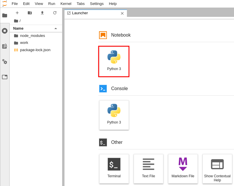
This creates an empty Jupyter notebook. From here, you can create code blocks called “cells,” which can be run selectively and will output the results of each execution below themselves once finished.
Authenticating with IBM Quantum
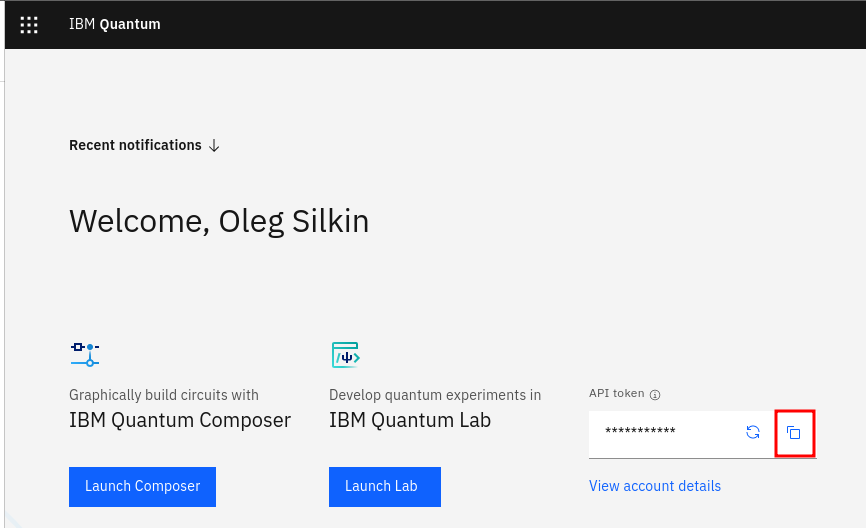
Before we begin constructing our circuits, we first need to authenticate ourselves with IBM Quantum backend. This will allow us to execute our circuits on both IBM’s Quantum Computers and Simulators. To obtain an API key from IBM Quantum, navigate to https://quantum-computing.ibm.com and log into your account (you’ll need to create an account if you do not already have one), then you will see your API key presented on the first page. Press the rightmost button to copy it into your clipboard:
Loading the token can be done in many ways:
- Placing the token directly into our code
- Pasting the token into a separate text file and then reading it into the program
- Setting it as an environment variable using .env (requires the python-dotenv library)
We will be focusing on the second method in this blog, since it does not require the usage of a third-party module.
With your API key copied into the clipboard, go ahead and press the plus button at the top-left of your Jupyter notebook window and select Text File at the new file menu:

Paste your API key into this file and save it as ibmq-key.txt . Then, navigate back to the Python notebook that you’re working in and run the following block of code to load it from the file:
### Using a file-read method
with open('ibmq-key.txt', 'r') as infile:
  ibmq_key = infile.read()
Next, import the IBMQ library from Qiskit and load the API key in:
from qiskit import IBMQ
# save account to your local machine (only need to do this once)
IBMQ.save_account(ibmq_key)
# load the account from the existing save
IBMQ.load_account()
# save the provider for later usage
provider = IBMQ.get_provider('ibm-q')
Now we will show how to build and run quantum circuits in the below examples. We will start with a basic Quantum-equivalent of “Hello World”, followed by a Quantum Random Number Generator and a Full-Adder.
1. Building quantum circuits: Hello World
Now that we have our environment configured, we can start building and executing real quantum circuits. We’ll begin by importing all of the things from Qiskit, as we’ll be using them extensively throughout this blog. To start building, let’s import all of the modules that we’ll need for this notebook:
import math
from matplotlib import style

from qiskit import *
from qiskit.tools.monitor import job_monitor
from qiskit.result import Result, Counts
from qiskit.providers.backend import Backend
from qiskit.visualization import plot_histogram
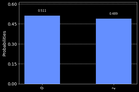
Our first circuit will be the quantum-equivalent of “Hello World” with the Qiskit SDK: calculating a simple coin toss. We accomplish this by placing a qubit in superposition and then measuring its state and recording the value into a classical register.
# quantum circuit with one qubit and one classical bit
num_qubits = 1
num_classical_bits = 1
coin_toss = QuantumCircuit(num_qubits, num_classical_bits)

# set an h-gate on the first qubit (0th index)
coin_toss.h(0)
# measure the value of the first qubit and place result into first cbit
coin_toss.measure([0,], [0,])
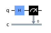
We can obtain a representation of the quantum circuit by using the QuantumCircuit.draw(output=’mpl’) method:
coin_toss.draw(output='mpl')
This will output a representation of our circuit rendered with matplotlib (hence the output=’mp’ kwarg):
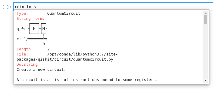
Pro tip for 1337 hackers: In Jupyter, you can view a drawing of your circuit anytime by placing your cursor on a QuantumCircuit object and pressing Shift+Tab:
Simulating our circuit
Now that we have created a quantum circuit and configured Qiskit to authenticate with our IBMQ account, our next step is to run our circuit on a quantum backend. For this tutorial, we will be using the simulator_statevector, since it is the recommended system for general-purpose quantum circuits (you can read more about it here: IBM Quantum simulators).
# use the statevector quantum simulator
backend = provider.get_backend("simulator_statevector")
job = execute(coin_toss, backend=backend, shots=8192)
# monitors the job and updates its status in real-time
job_monitor(job)
To minimize the amount of variation in our results, we’ll execute the circuit 8,192 times by providing the shots=8192 kwarg (Python lingo for keyword argument).
After the job completes, we’ll visualize the results from job.result() using matplotlib:
# display the results from the job
style.use("dark_background")
result = job.result()

counts = result.get_counts(coin_toss)
plot_histogram([counts])
Running the above code produces the following histogram:
2. Building quantum circuits: quantum random number generator
An extremely useful property of quantum computers is that they are a source of pure randomness. By the laws of quantum mechanics, qubit in superposition will collapse to either 0 or 1 with equal probability, meaning that we will never be able to predict its value ahead of time. We can make use of this property by constructing a circuit to place a series of qubits in superposition, measure their values, and then concatenate the results to produce a completely random number.
We’ll start by creating a circuit of a parameterized number of qubits, with a hadamard gate being applied to each of them:
def quantum_rng(n: int) -> QuantumCircuit:
 qb = QuantumRegister(n, 'q-random-bit')
 cr = ClassicalRegister(n, 'measured-random-bit')
 qc = QuantumCircuit(qb, cr)
 qc.h(qb)
 qc.measure(qb, cr)
 return qc
We can then configure our circuit to run a bunch of times, joining the results together in order to get a large random number. The bit size that we can generate each time is equal to the number of available qubits multiplied by the amount of shots we run the circuit through: #bits = #qubits * #shots
def execute_circuit_ibmq(qc: QuantumCircuit, backend: Backend, shots: int = 8096) -> Counts | None:
 counts = None
 job = execute(qc, backend=backend, shots=shots)
 job_monitor(job)
 result = job.result()
 counts = result.get_counts(qc)
 return counts

def generate_random_number(n_bits: int=4096, backend: Backend=None) -> int:
 # to generate more bits, we just run a ton of shots & truncate to the appropriate length
 n_qubits = backend.configuration().n_qubits
 n_shots = math.ceil(n_bits / n_qubits)
 # for small numbers, only run once & grab the requested amount of bits
 if n_bits < n_qubits:
   n_qubits = n_bits

 qc = quantum_rng(n_qubits)
 counts = execute_circuit_ibmq(qc, backend, n_shots)
 # add each binary string to the huge string of binary numbers
 # until every binary string has a count of 0 in the counts
 binary_number = ''
 bstr_stack = list(counts.keys())
 while len(bstr_stack) > 0:
   bstr = bstr_stack.pop()
   binary_number += bstr
   counts[bstr] -= 1
   if counts[bstr] == 0:
     continue
   else:
     bstr_stack.append(bstr)
 # trim the binary_number to be the exact length in bits
 if len(binary_number) > n_bits:
   binary_number = binary_number[:n_bits]

 num = int(binary_number, 2)
 return num
The above code accepts a bit amount and a selected backend from which it determines how many times it needs to execute before we have enough information to form a number of the requested bit count. Let’s use the simulator_statevector to generate a 2048-bit integer:
random_num = generate_random_number(2048, backend)
Computing the base-2 log of our random_num shows that we received a number which has roughly 2048 bits:
math.log2(random_num)
Of course, the above code isn’t truly random since the operations are still performed using classical simulations. For true randomness, we can run this through a real quantum machine, although the queues are significantly longer on average when compared to the simulators:
# running the quantum random number generator on a real quantum computer
provider = IBMQ.get_provider('ibm-q')
backend = provider.get_backend('ibmq_quito')
quantum_random_num = generate_random_number(2048, backend)
3. Building quantum circuits: full-adder
In the world of computational logic, a full-adder is a circuit which takes in three values as input: A, B, and Cin; where A and B are the numbers to be added, and Cin is a carry-over bit to determine whether we must carry an extra number into our computation. A full-adder has two outputs: sum and carry, which determine the sum of the two numbers, and whether we must carry over, respectively. We can express these two values via the following logic equations:
Sum = (A XOR B) XOR C
Carry = (C AND (A XOR B)) OR (A AND B)
The following code implements the logic for a full-adder in Qiskit:
def sum_bit(qc: QuantumCircuit, a: int, b: int, c: int, out0: int, out1: int):
 # A xor B
 qc.cx(a, out0)
 qc.cx(b, out0)

 # (A XOR B) XOR C
 qc.cx(out0, out1)
 qc.cx(c, out1)

def carry_bit(qc: QuantumCircuit, a: int, b: int, c: int, q0: int, q2: int, q3: int, q4: int):
 # Use the DeMorgan's Law for the OR gate: A OR B = NOT (NOT A AND NOT B)

 # NOT (C AND (A XOR B))
 qc.ccx(c, q0, q2)
 qc.x(q2)

 # NOT (A AND B)
 qc.ccx(a, b, q3)
 qc.x(q3)

 # NOT ( NOT(A AND B) AND NOT(C AND (A XOR B)))
 qc.ccx(q3, q2, q4)
 qc.x(q4)


# Quantum Full-Adder
def full_adder(a: int=0, b: int=0, cin: int=0) -> QuantumCircuit:
 qc = QuantumCircuit(8, 2)

 # Initialize A, B, and C
 if a == 1:
   qc.x(0)
 if b == 1:
   qc.x(1)
 if cin == 1:
   qc.x(2)

 qc.barrier()
  # Sum bit
 sum_bit(qc, 0, 1, 2, 3, 4)
 qc.barrier()

 # Carry bit
 carry_bit(qc, 0, 1, 2, 3, 5, 6, 7)
 qc.barrier()

 # Measure
 qc.measure(4, 0)
 qc.measure(7, 1)

 return qc
We can run the above code using varying values for A, B, and C to verify that we indeed get the output corresponding to the appropriate entry in the logic table for a full-adder:
| A | B | Cin | Sum | Carry |
| 0 | 0 | 0 | 0 | 0 |
| 1 | 0 | 0 | 1 | 0 |
| 0 | 1 | 0 | 1 | 0 |
| 1 | 1 | 0 | 0 | 1 |
| 0 | 0 | 1 | 1 | 0 |
| 1 | 0 | 1 | 0 | 1 |
| 0 | 1 | 1 | 0 | 1 |
| 1 | 1 | 1 | 1 | 1 |
We can run our circuit against the tautology table above to verify the validity of our circuit.
tautology_table = {}
# perform a tautology on the full-adder
for a in [0, 1]:
 for b in [0, 1]:
   for c in [0, 1]:
     qc = full_adder(a, b, c)
     job = execute(qc, backend=backend, shots=1)
     job_monitor(job)
     result = job.result()
     counts = result.get_counts(qc)
     count_str = list(counts.keys())[0]
     sum_reg = int(count_str[1])
     count_reg = int(count_str[0])
     tautology_table[(a, b, c)] = (sum_reg, count_reg)

# print each entry on a newline
for key, value in tautology_table.items():
 print(f'{key}: {value}')
Running the above code should result in the following table:
(0, 0, 0): (0, 0)
(0, 0, 1): (1, 0)
(0, 1, 0): (1, 0)
(0, 1, 1): (0, 1)
(1, 0, 0): (1, 0)
(1, 0, 1): (0, 1)
(1, 1, 0): (0, 1)
(1, 1, 1): (1, 1)
Congratulations! You have just created your very first quantum arithmetic module. Though it may be very basic, the concepts introduced in the previous few examples can be elaborated on to create larger and more complex circuits to serve important applications such as developing medicines, securing data transfer, and finding the most optimal shortest path, to name just a few.
Summary
To summarize, we have just learned that we can use Qiskit to build and execute quantum circuits in OpenShift through the following procedure:
- Install the QiskitPlayground operator in an OpenShift cluster
- Create an instance of QiskitPlayground
- Access JupyterLab through the route created by QiskitPlayground
- Obtain an API Key for IBM Quantum and save it with the Qiskit SDK
- Build a quantum circuit using the Qiskit SDK
- Execute the quantum circuit in an IBM simulator
Our next blog post will investigate how IBM Quantum can be leveraged to execute circuits on real quantum computers provided by IBMQ’s backend.
If you reached the end of this blog and are still hungry for more quantum computing, here are some awesome quantum circuits to check out:
https://qiskit.org/textbook/ch-labs/Lab01_QuantumCircuits.html
https://qiskit.org/documentation/apidoc/circuit.html
https://qiskit.org/documentation/tutorials/circuits/1_getting_started_with_qiskit.html
Qiskit also has a fantastic video series demonstrating how these circuits are built up:
https://www.youtube.com/watch?v=a1NZC5rqQD8&list=PLOFEBzvs-Vvp2xg9-POLJhQwtVktlYGbY